Chapter 4: RAN Internals¶

4.1 Packet Processing Pipeline¶

Figure 4.1 shows the packet processing stages implemented by the base station. These stages are specified by the 3GPP standard. Note that the figure depicts the base station as a pipeline (running left-to-right) but it is equally valid to view it as a protocol stack (as is typically done in official 3GPP documents). Also note that (for now) we are agnostic as to how these stages are implemented, but since we are ultimately heading towards a cloud-based implementation, you can think of each as corresponding to a microservice (if that is helpful).

Figure 4.1: RAN processing pipeline, including both user and control plane components.

The key stages are as follows:

• RRC (Radio Resource Control) → Responsible for configuring the coarse-grain and policy-related aspects of the pipeline. The RRC runs in the RAN’s control plane; it does not process packets on the user plane.
• PDCP (Packet Data Convergence Protocol) → Responsible for compressing and decompressing IP headers, ciphering and integrity protection, and making an “early” forwarding decision (i.e., whether to send the packet down the pipeline to the UE or forward it to another base station).
• RLC (Radio Link Control) → Responsible for segmentation and reassembly, including reliably transmitting/receiving segments by implementing ARQ.
• MAC (Media Access Control) → Responsible for buffering, multiplexing and demultiplexing segments, including all real-time scheduling decisions about what segments are transmitted when. Also able to make a “late” forwarding decision (i.e., to alternative carrier frequencies, including Wi-Fi).
• PHY (Physical Layer) → Responsible for coding and modulation (as discussed in an earlier chapter), including FEC.

The last two stages in Figure 4.1 (D/A conversion and the RF front-end) are beyond the scope of this book.

While it is simplest to view the stages in Figure 4.1 as a pure left-to-right pipeline, in practice the Scheduler running in the MAC stage implements the “main loop” for outbound traffic, reading data from the upstream RLC and scheduling transmissions to the downstream PHY. In particular, since the Scheduler determines the number of bytes to transmit to a given UE during each time period (based on all the factors outlined in an earlier chapter), it must request (get) a segment of that length from the upstream queue. In practice, the size of the segment that can be transmitted on behalf of a single UE during a single scheduling interval can range from a few bytes to an entire IP packet.

4.2 Split RAN¶

The next step is understanding how the functionality outlined above is partitioned between physical elements, and hence, “split” across centralized and distributed locations. Although the 3GPP standard allows for multiple split-points, the partition shown in Figure 4.2 is the one being actively pursued by the operator-led O-RAN (Open RAN) Alliance. It is the split we adopt throughout the rest of this book.

Figure 4.2: Split-RAN processing pipeline distributed across a Central Unit (CU), Distributed Unit (DU), and Radio Unit (RU).

This results in a RAN-wide configuration similar to that shown in Figure 4.3, where a single Central Unit (CU) running in the cloud serves multiple Distributed Units (DUs), each of which in turn serves multiple Radio Units (RUs). Critically, the RRC (centralized in the CU) is responsible for only near-real time configuration and control decision making, while the Scheduler that is part of the MAC stage is responsible for all real-time scheduling decisions.

Figure 4.3: Split-RAN hierarchy, with one CU serving multiple DUs, each of which serves multiple RUs.

Clearly, a DU needs to be “near” (within 1ms) the RUs it manages since the MAC schedules the radio in real-time. One familiar configuration is to co-locate a DU and an RU in a cell tower. But when an RU corresponds to a small cell, many of which might be spread across a modestly sized geographic area (e.g., a mall, campus, or factory), then a single DU would likely service multiple RUs. The use of mmWave in 5G is likely to make this later configuration all the more common.

Also note that the split-RAN changes the nature of the Backhaul Network, which in 4G connected the base stations (eNBs) back to the Mobile Core. With the split-RAN there are multiple connections, which are officially labelled as follows:

• RU-DU connectivity is called the Fronthaul
• DU-CU connectivity is called the Midhaul
• CU-Mobile Core connectivity is called the Backhaul

As we will see in a later chapter, one possible deployment co-locates the CU and Mobile Core in the same cluster, meaning the backhaul is implemented in the cluster switching fabric. In such a configuration, the midhaul then effectively serves the same purpose as the original backhaul, and the fronthaul is constrained by the predictable/low-latency requirements of the MAC stage’s real-time scheduler.

4.3 Software-Defined RAN¶

Finally, we describe how the RAN is implemented according to SDN principles, resulting in an SD-RAN. The key architectural insight is shown in Figure 4.4, where the RRC from Figure 4.1 is partitioned into two sub-components: the one on the left provides a 3GPP-compliant way for the RAN to interface to the Mobile Core’s control plane, while the latter opens a new programmatic API for exerting software-based control over the pipeline that implements the RAN user plane. To be more specific, the left sub-component simply forwards control packets between the Mobile Core and the PDCP, providing a path over which the Mobile Core can communication with the UE for control purposes, whereas the right sub-component implements the core of the RCC’s control functionality.

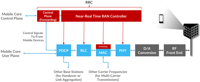
Figure 4.4: RRC disaggregated into a Mobile Core facing control plane component and a Near Real-Time Controller.

Although not shown in Figure 4.4, keep in mind (from Figure 4.2) that all constituent parts of the RRC, plus the PDCP, form the CU.

Completing the picture, Figure 4.5 shows the Near-RT RAN Controller implemented as a traditional SDN Controller hosting a set of SDN control apps. The Near Real-Time Controller maintains a RAN Network Information Base (R-NIB) that includes time-averaged CQI values and other per-session state (e.g., GTP tunnel IDs, QCI values for the type of traffic), while the MAC (as part of the DU) maintains the instantaneous CQI values required by the real-time scheduler. Specifically, the R-NIB includes the following state:

• NODES: Base Stations and Mobile Devices
  • Base Station Attributes:
    • Identifiers
    • Version
    • Config Report
    • RRM config
    • PHY resource usage
  • Mobile Device Attributes:
    • Identifiers
    • Capability
    • Measurement Config
    • State (Active/Idle)
• LINKS: Physical between two nodes and potential between UEs and all neighbor cells
  • Link Attributes:
    • Identifiers
    • Link Type
    • Config / Bearer Parameters
    • QCI Value
• SLICES: Virtualized RAN construct
  • Slice Attributes:
    • Links
    • Bearers / Flows
    • Validity Period
    • Desired KPIs
    • MAC RRM Configuration
    • RRM Control Configuration

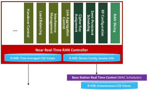
Figure 4.5: Example set of control applications running on top of Near Real-Time RAN Controller.

The example Control Apps in Figure 4.5 include a range of possibilities, but is not intended to be an exhaustive list. The right-most example, RAN Slicing, is the most ambitious in that it introduces a new capability: Virtualizing the RAN. It is also an idea that has been implemented, which we describe in more detail in the next chapter.

The next three (RF Configuration, Semi-Persistent Scheduling, Cipher Key Assignment) are examples of configuration-oriented applications. They provide a programmatic way to manage seldom-changing configuration state, thereby enabling zero-touch operations. Coming up with meaningful policies (perhaps driven by analytics) is likely to be an avenue for innovation in the future.