Chapter 5: Advanced Capabilities¶

5.1 Optimized Data Plane¶

There are many reasons to disaggregate functionality, but one of the most compelling is that by decoupling control and data code paths, it is possible to optimize the data path. This can be done, for example, by programming it into specialized hardware. Modern white-box switches with programmable packet forwarding pipelines are a perfect example of specialized hardware we can exploit in the cellular network. Figure 5.1 shows the first step in the process of doing this. The figure also pulls together all the elements we’ve been describing up to this point. There are several things to note about this diagram.

Figure 5.1: End-to-end disaggregated system, including Mobile Core and Split-RAN.

First, the figure combines both the Mobile Core and RAN elements, organized according to the major subsystems: Mobile Core, Central Unit (CU), Distributed Unit (DU), and Radio Unit (RU). The figure also shows one possible mapping of these subsystems onto physical locations, with the first two co-located in a Central Office and the latter two co-located in a cell tower. As discussed earlier, other configurations are also possible.

Second, the figure shows the Mobile Core’s two user plane elements (PGW, SGW) and the Central Unit’s single user plane element (PDCP) further disaggregated into control/user plane pairs, denoted PGW-C / PGW-U, SGW-C / SGW-U, and PDCP-C / PDCP-U, respectively. Exactly how this decoupling is realized is a design choice (i.e., not specified by 3GPP), but the idea is to reduce User Plane component to the minimal Receive-Packet / Process-Packet / Send-Packet processing core, and elevate all control-related aspects into the Control Plane component.

Third, the PHY (Physical) element of the RAN pipeline is split between the DU and RU partition. Although beyond the scope of this book, the 3GPP spec specifies the PHY element as a collection of functional blocks, some of which can be effectively implemented by software running on a general-purpose processor and some of which are best implemented in specialized hardware (e.g., a Digital Signal Processor). These two subsets of functional blocks map to the PHY Upper (part of the DU) and the PHY Lower (part of the RU), respectively.

Fourth, and somewhat confusingly, Figure 5.1 shows the PCDP-C element and the Control Plane (Forwarding) element combined into a single functional block, with a data path (blue line) connecting that block to both the RLC and the MME. Exactly how this pair is realized is an implementation choice (e.g., they could map onto two or more microservices), but the end result is that they are part of an end-to-end path over which the MME can send control packets to the UE. Note that this means responsibility for demultiplexing incoming packets between the control plane and user plane falls to the RLC.

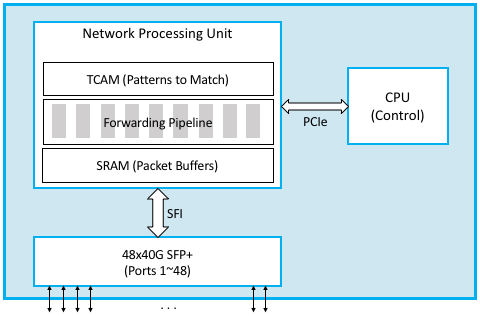
Figure 5.2: Implementing data plane elements of the User Plane in programmable switches.

Figure 5.2 shows why we disaggregated these components: it allows us to realize the three user plane elements (PGW-U, SGW-U, PDCP-U) in switching hardware. This can be done using a combination of a language that is tailored for programming forwarding pipelines (e.g., P4), and a protocol-independent switching architecture (e.g., Tofino). For now, the important takeaway is that the RAN and Mobile Core user plane can be mapped directly onto an SDN-enabled data plane.

Pushing RAN and Mobile Core forwarding functionality into the switching hardware results in overlapping terminology that can sometimes be confusing. 5G separates the functional blocks into control and user planes, while SDN disaggregates a given functional block into control and data plane halves. The overlap comes from our choosing to implement the 5G user plane by splitting it into its SDN-based control and data plane parts. As one simplification, we refer to the Control Plane (Forwarding) and PDCP-C combination as the CU-C (Central Unit - Control) going forward.

Finally, the SDN-prescribed control/data plane disaggregation comes with an implied implementation strategy, namely, the use of a scalable and highly available Network Operating System (NOS). Like a traditional OS, a NOS sits between application programs (control apps) and the underlying hardware devices (whitebox switches), providing higher levels abstractions (e.g., network graph) to those applications, while hiding the low-level details of the underlying hardware. To make the discussion more concrete, we use ONOS (Open Network Operating System) as an example NOS, where PGW-C, SGW-C, and PDCP-C are all realized as control applications running on top of ONOS.

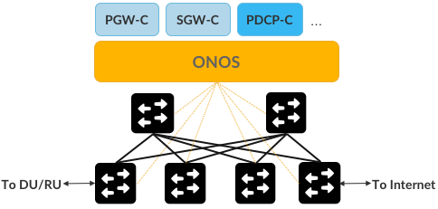
Figure 5.3: Control Plane elements of the User Plane implemented as Control Applications running on an SDN Controller (e.g., ONOS).

Figure 5.3 shows one possible configuration, in which the underlying switches are interconnected to form a leaf-spine fabric. Keep in mind that the linear sequence of switches implied by Figure 5.2 is logical, but that in no way restricts the actual hardware to the same topology. The reason we use a leaf-spine topology is related to our ultimate goal of building an edge cloud, and leaf-spine is the proto-typical structure for such cloud-based clusters. This means the three control applications must work in concert to implement an end-to-end path through the fabric, which in practice happens with the aid of other, fabric aware, control applications (as implied by the “…” in the Figure). We describe the complete picture in more detail in the next chapter, but for now, the big takeaway is that the control plane components of the 5G overlay can be realized as control applications for an SDN-based underlay.

5.2 Multi-Cloud¶

Another consequence of disaggregating functionality is that once decoupled, different functions can be placed in different physical locations. We have already seen this when we split the RAN, placing some functions (e.g., the PCDP and RRC) in the Central Unit and others (e.g., RLC and MAC) in Distributed Units. This allows for simpler (less expensive) hardware in remote locations, where there are often space, power, and cooling constraints.

This process can be repeated by distributing the more centralized elements across multiple clouds, including large datacenters that already benefit from elasticity and economies of scale. Figure 5.4 shows the resulting multi-cloud realization of the Mobile Core. We leave the user plane at the edge of the network (e.g., in the Central Office) and move control plane to a centralized cloud. It could even be a public cloud like Google or Amazon. This includes not only the MME, PCRF and HSS, but also the PGW-C and SGW-C we decoupled in the previous section. (Note that Figure 5.4 renames the PDCP-U from earlier diagrams as the CU-U; either label is valid.)

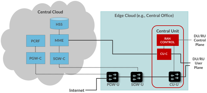
Figure 5.4: Multi-Cloud implementation, with MME, HSS, PCRF and Control Plane elements of the PGW and SGW running in a centralized cloud.

What is the value in doing this? Just like the DU and RU, the Edge Cloud likely has limited resources. If we want room to run new edge services there, it helps to move any components that need not be local to a larger facility with more abundant resources. Centralization also facilitates collecting and analyzing data across multiple edge locations, which is harder to do if that information is distributed over multiple sites. (Analytics performed on this data also benefits from having abundant compute resources available.)

But there’s another reason worth calling out: It lowers the barrier for anyone (not just the companies that own and operate the RAN infrastructure) to offer mobile services to customers. These entities are called MVNOs (Mobile Virtual Network Operators) and one clean way to engineer an MVNO is to run your own Mobile Core on a cloud of your choosing.

5.3 Network Slicing¶

One of the most compelling value propositions of 5G is the ability to differentiate the level of service offered to different applications and customers. Differentiation, of course, is key to being able to charge some customers more than others, but the monetization case aside, it is also necessary if you are going to support such widely varying applications as streaming video (which requires high bandwidth but can tolerate larger latencies) and Internet-of-Things (which has minimal bandwidth needs but requires extremely low and predictable latencies).

The mechanism that supports this sort of differentiation is called network slicing, and it fundamentally comes down to scheduling, both in the RAN (deciding which segments to transmit) and in the Mobile Core (scaling microservice instances and placing those instances on the available servers). The following introduces the basic idea, starting with the RAN.

But before getting into the details, we note that a network slice is a generalization of the QoS Class Index (QCI) discussed earlier. 3GPP specifies a standard set of network slices, called Standardized Slice Type (SST) values. For example, SST 1 corresponds to mobile broadband, SST 2 corresponds to Ultra-Reliable Low Latency Communications, SST 3 corresponds to Massive IoT, and so on. It is also possible to extend this standard set with additional slice behaviors, as well as define multiple slices for each SST (e.g., to further differentiate subscribers based on priority).

RAN Slicing¶

We start by reviewing the basic scheduling challenge previewed in Chapter 2. As depicted in Figure 5.5, the radio spectrum can be conceptualized as a two-dimensional grid of Resource Blocks (RB), where the scheduler’s job is to decide how to fill the grid with the available segments from each user’s transmission queue based on CQI feedback from the UEs. To restate, the power of OFDMA is the flexibility it provides in how this mapping is performed.

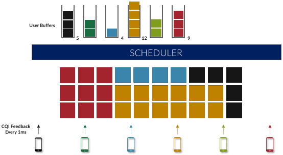
Figure 5.5: Scheduler allocating resource blocks to UEs.

While in principle one could define an uber scheduler that takes dozens of different factors into account, the key to network slicing is to add a layer of indirection, such that (as shown in Figure 5.6, we perform a second mapping of Virtual RBs to Physical RBs. This sort of virtualization is common in resource allocators throughout computing systems because we want to separate how many resources are allocated to each user from the decision as to which physical resources are actually assigned. This virtual-to-physical mapping is performed by a layer typically known as a Hypervisor, and the important thing to keep in mind is that it is totally agnostic about which user’s segment is affected by each translation.

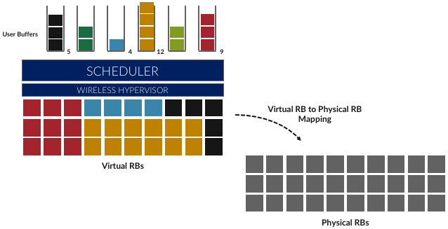
Figure 5.6: Wireless Hypervisor mapping virtual resource blocks to physical resource blocks.

Having decoupled the Virtual RBs from Physical RBs, it is now possible to define multiple Virtual RB sets (of varying sizes), each with its own scheduler. Figure 5.7 gives an example with two equal-sized RB sets, where the important consequence is that having made the macro-decision that the Physical RBs are divided into two equal partitions, the scheduler associated with each partition is free to allocate Virtual RBs completely independent from each other. For example, one scheduler might be designed to deal with high-bandwidth video traffic and another scheduler might be optimized for low-latency IoT traffic. Alternatively, a certain fraction of the available capacity could be reserved for premium customers or other high-priority traffic (e.g., public safety), with the rest shared among everyone else.

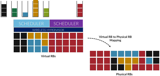
Figure 5.7: Multiple schedulers running on top of wireless hypervisor.

Going one level deeper in the implementation details, the real-time scheduler running in each DU receives high-level directives from the near real-time scheduler running in the CU, and as depicted in Figure 5.8, these directives make dual transmission, handoff, and interference decisions on a per-slice basis. A single RAN Slicing control application is responsible for the macro-scheduling decision by allocating resources among a set of slices. Understanding this implementation detail is important because all of these control decisions are implemented by software modules, and hence, easily changed or customized. They are not “locked” into the underlying system, as they have historically been in 4G’s eNodeBs.

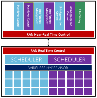
Figure 5.8: Centralized near-realtime control applications cooperating with distribute real-time RAN schedulers.