Chapter 2: Radio Transmission¶

2.1 Coding and Modulation¶

The mobile channel over which digital data needs to be reliably transmitted brings a number of impairments, including noise, attenuation, distortion, fading, and interference. This challenge is addressed by a combination of coding and modulation, as depicted in Figure 2.1.

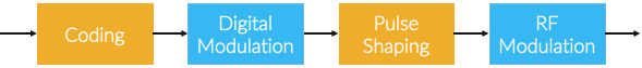
Figure 2.1: The role of coding and modulation in mobile communication.

At its core, coding inserts extra bits into the data to help recover from all the environmental factors that interfere with signal propagation. This typically implies some form of Forward Error Correction (e.g., turbo codes, polar codes). Modulation then generates signals that represent the encoded data stream, and it does so in a way that matches the channel characteristics: It first uses a digital modulation signal format that maximizes the number of reliably transmitted bits every second based on the specifics of the observed channel impairments; it next matches the transmission bandwidth to channel bandwidth using pulse shaping; and finally, it uses RF modulation to transmit the signal as an electromagnetic wave over an assigned carrier frequency.

For a deeper appreciation of the challenges of reliably transmitting data by propagating radio signals through the air, consider the scenario depicted in Figure 2.2, where the signal bounces off various stationary and moving objects, following multiple paths from the transmitter to the receiver, who may also be moving.

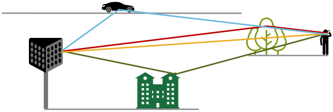
Figure 2.2: Signals propagate along multiple paths from transmitter to receiver.

As a consequence of these multiple paths, the original signal arrives at the receiver spread over time, as illustrated in Figure 2.3. Empirical evidence shows that the Multipath Spread—the time between the first and last signals of one transmission arriving at the receiver—is 1 to 10μs in urban environments and 10 to 30μs in suburban environments. Theoretical bounds for the time duration for which the channel may be assumed to be time invariant, known as the Coherence Time and denoted \(T_c\), is given by

where \(c\) is the velocity of the signal, \(v\) is the velocity of the receiver (e.g., moving car or train), and \(f\) is the frequency of the carrier signal that is being modulated. This says the coherence time is inversely proportional to the frequency of the signal and the speed of movement, which makes intuitive sense: The higher the frequency (narrower the wave) the shorter the coherence time, and likewise, the faster the receiver is moving the longer the coherence time. Based on the target parameters to this model (selected according to the target physical environment), it is possible to calculate \(T_c\), which in turn bounds the rate at which symbols can be transmitted without undue risk of interference.

Figure 2.3: Received data spread over time due to multipath variation.

To complicate matters further, Figure 2.2 and 2.3 imply the transmission originates from a single antenna, but cell towers are equipped with an array of antennas, each transmitting in a different (but overlapping) direction. This technology, called Multiple-Input-Multiple-Output (MIMO), opens the door to purposely transmitting data from multiple antennas in an effort to reach the receiver, adding even more paths to the environment-imposed multipath propagation.

One of the most important consequences of these factors is that the transmitter must receive feedback from every receiver to judge how to best utilize the wireless medium on their behalf. 3GPP specifies a Channel Quality Indicator (CQI) for this purpose, where in practice the receiver sends a CQI status report to the base station periodically (e.g., every millisecond in LTE). These CQI messages report the observed signal-to-noise ratio, which impacts the receiver’s ability to recover the data bits. The base station then uses this information to adapt how it allocates the available radio spectrum to the subscribers it is serving, as well as which coding and modulation scheme to employ. All of these decisions are made by the scheduler.

How the scheduler does its job is one of the most important properties of each generation of the cellular network, which in turn depends on the multiplexing mechanism. For example, 2G used Time Division Multiple Access (TDMA) and 3G used Code Division Multiple Access (CDMA). It is also a major differentiator for 4G and 5G, completing the transition from the cellular network being fundamentally circuit-switched to fundamentally packet-switched. The following two sections describe each, in turn.

2.2 Scheduling: 4G¶

The state-of-the-art in multiplexing 4G cellular networks is called Orthogonal Frequency-Division Multiple Access (OFDMA). The idea is to multiplex data over a set of 12 orthogonal subcarrier frequencies, each of which is modulated independently. The “Multiple Access” in OFDMA implies that data can simultaneously be sent on behalf of multiple users, each on a different subcarrier frequency and for a different duration of time. The subbands are narrow (e.g., 15kHz), but the coding of user data into OFDMA symbols is designed to minimize the risk of data loss due to interference between adjacent bands.

The use of OFDMA naturally leads to conceptualizing the radio spectrum as a two-dimensional resource, as shown in Figure 2.4. The minimal schedulable unit, called a Resource Element (RE), corresponds to a 15kHz-wide band around one subcarrier frequency and the time it takes to transmit one OFDMA symbol. The number of bits that can be encoded in each symbol depends on the modulation rate, so for example using Quadrature Amplitude Modulation (QAM), 16-QAM yields 4 bits per symbol and 64-QAM yields 16 bits per symbol

Figure 2.4: Spectrum abstractly represented by a 2-D grid of schedulable Resource Elements.

A scheduler allocates some number of REs to each user that has data to transmit during each 1ms Transmission Time Interval (TTI, where users are depicted by different colored blocks in Figure 2.4. The only constraint on the scheduler is that it must make its allocation decisions on blocks of 7x12=84 resource elements, called a Physical Resource Block (PRB). Figure 2.4 shows two back-to-back PRBs. Of course time continues to flow along one axis, and depending on the size of the available frequency band (e.g., it might be 100MHz wide), there may be many more subcarrier slots (and hence PRBs) available along the other axis, so the scheduler is essentially preparing and transmitting a sequence of PRBs.

Note that OFDMA is not a coding/modulation algorithm, but instead provides a framework for selecting a specific coding and modulator for each subcarrier frequency. QAM is one common example modulator. It is the scheduler’s responsibility to select the modulation to use for each PRB, based on the CQI feedback it has received. The scheduler also selects the coding on a per-PRB basis, for example, by how it sets the parameters to the turbo code algorithm.

The 1ms TTI corresponds to the time frame in which the scheduler receives feedback from users about the quality of the signal they are experiencing. This is the CQI mentioned earlier, where once every millisecond, each user sends a set of metrics, which the scheduler uses to make its decision as to how to allocate PRBs during the subsequent TTI.

Another input to the scheduling decision is the QoS Class Identifier (QCI), which indicates the quality-of-service each class of traffic is to receive. In 4G, the QCI value assigned to each class (there are nine such classes, in total) indicates whether the traffic has a Guaranteed Bit Rate (GBR) or not (non-GBR), plus the class’s relative priority within those two categories.

Finally, keep in mind that Figure 2.4 focuses on scheduling transmissions from a single antenna, but the MIMO technology described above means the scheduler also has to determine which antenna (or more generally, what subset of antennas) will most effectively reach each receiver. But again, in the abstract, the scheduler is charged with allocating a sequence of Resource Elements.

This all begs the question: How does the scheduler decide which set of users to service during a given time interval, how many resource elements to allocate to each such user, how to select the coding and modulation levels, and which antenna to transmit their data on? This is an optimization problem that, fortunately, we are not trying to solve here. Our goal is to describe an architecture that allows someone else to design and plug in an effective scheduler. Keeping the cellular architecture open to innovations like this is one of our goals, and as we will see in the next section, becomes even more important in 5G where the scheduler operates with even more degrees of freedom.

2.3 Scheduling: 5G¶

The transition from 4G to 5G introduces additional degrees-of-freedom in how the radio spectrum is scheduled, making it possible to adapt the cellular network to a more diverse set of devices and applications domains.

Fundamentally, 5G defines a family of waveforms—unlike LTE, which specified only one waveform—each optimized for a different band in the radio spectrum. The bands with carrier frequencies below 1GHz are designed to deliver mobile broadband and massive IoT services with a primary focus on range. Carrier frequencies between 1GHz-6GHz are designed to offer wider bandwidths, focusing on mobile broadband and mission-critical applications. Carrier frequencies above 24GHz (mmWaves) are designed to provide super wide bandwidths over short, line-of-sight coverage.

These different waveforms affect the scheduling and subcarrier intervals (i.e., the “size” of the resource elements described in the previous section).

• For sub-1GHz bands, 5G allows maximum 50MHz bandwidths. In this case, there are two waveforms: one with subcarrier spacing of 15kHz and another of 30kHz. (We used 15kHz in the example shown in Figure 2.4.) The corresponding scheduling intervals are 0.5ms and 0.25ms, respectively. (We used 0.5ms in the example shown in Figure 2.4.)
• For 1GHz-6GHz bands, maximum bandwidths go up to 100MHz. Correspondingly, there are three waveforms with subcarrier spacings of 15kHz, 30kHz and 60kHz, corresponding to scheduling intervals of 0.5ms, 0.25ms and 0.125ms, respectively.
• For millimeter bands, bandwidths may go up to 400MHz. There are two waveforms, with subcarrier spacings of 60kHz and 120kHz. Both have scheduling intervals of 0.125ms.

This range of options is important because it adds another degree of freedom to the scheduler. In addition to allocating radio resources to users, it has the ability to dynamically adjust the size of the resource by changing the wave form being used. With this additional freedom, fixed-sized REs are no longer the primary unit of resource allocation. We instead use more abstract terminology, and talk about allocating Resource Blocks to subscribers, where the 5G scheduler determines both the size and number of Resource Blocks allocated during each time interval.

Figure 2.5 depicts the role of the scheduler from this more abstract perspective, where just as with 4G, CQI feedback from the receivers and the QCI quality-of-service class selected by the subscriber are the two key pieces of input to the scheduler. Note that the set of QCI values changes between 4G and 5G, reflecting the increasing differentiation being supported. For 5G, each class includes the following attributes:

• Resource Type: Guaranteed Bit Rate (GBR), Delay-Critical GBR, Non-GBR
• Priority Level
• Packet Delay Budget
• Packet Error Rate
• Averaging Window
• Maximum Data Burst

Note that while the preceding discussion could be interpreted to imply a one-to-one relationship between subscribers and a QCI, it is more accurate to say that each QCI is associated with a class of traffic (often corresponding to some type of application), where a given subscriber might be sending and receiving traffic that belongs to multiple classes at any given time. We explore this idea in much more depth in a later chapter.

Figure 2.5: Scheduler allocates Resource Elements to user data streams based on CQI feedback from receivers and the QCI parameters associated with each class of service.